The price of call options relative to the fair price means that deep in-the-money call options are not a good solution for achieving 300% leverage as might be desired for effective altruism investing.
Deep in-the-money call options are more complex to invest in and are expected to perform worse than small cap value.
This article expands on Effective Altruism Investing Strategies by looking at the suitability of stock options for effective altruism investments. In particular, I consider the use of in-the-money call options as a means of obtaining leverage.
Effective altruism is a movement that seeks to use reason to achieve the most good in the world.
Leverage is an advanced investing topic, and leverage should only be considered if you have mastered other aspects of investing, especially the potential permanently negative consequences of taking on risk.
Call and put options give you the right, but not the obligation, to buy or sell a particular stock at a particular price, called the strike price, on, or possibly before, some date. European style options only allow exercise on some date. American style options allow exercise on or before some date. Options are normally sold on or before their expiration and settled in cash, not exercised for shares.
By purchasing long-term in-the-money calls it is possible to obtain a leveraged position. For instance you might pay $30 for a call option which gives you the right to buy next year for $80 a stock that is currently trading at $100. If the price of the underlying stock moves up by a dollar, the value of the option will also increase by close to a dollar. In other words a 1% increase in the stock price produced approximately a 3% increase in the option price. Options are also available on stock indexes. Stock options on the S&P 500 are particularly heavily traded, making them a prime opportunity for obtaining leverage.
The advantages of using call options for leverage are you don't have to pay margin interest, and it is impossible to lose more than you have invested. The downside is the bid-ask spread, having to roll over the position every year or so, and whether the options are fairly priced.
Rolling positions frequently has the benefit of maintaining the target level of risk. If stocks move up the leverage factor declines, reducing returns, while if stocks move down the amount of leverage may become too great introducing the possibility of the position being wiped out. To avoid getting wiped out with longer option durations requires continual monitoring, and if stocks ever drop by too much selling the position and establishing a new less leveraged position.
Options on the S&P 500 come in several flavors, none of which are ideal. SPX and SPXW options trade in units of 100 times the S&P index value. This means a single deep in-the-money call option might cost around $100,000. XSP mini-options are one tenth the size of SPX options, but aren't available as 2-3 year-long dated LEAP options. And SPY ETF options which are American style options and are settled in ETF shares rather than cash. At least for longer durations, the bid-ask spreads on SPX often appear better than those on SPXW.
It should be noted that options on indexes, but probably not on ETFs, receive special tax treatment in the U.S. in accordance with Section 1256. Briefly, the option position is marked to market at the end of the year, and even though commonly held for less than a year, 60% of any gains are treated as long term capital gains, with the remainder treated as short term capital gains. Losses can be carried back for up to 3 years.
For my analysis I attempt to use SPX options and their predecessor options exclusively. They have reasonably tight spreads, and because they are European style options are easy to value.
The fair price of European style options is determined using the Black-Scholes model. A key input into the model is the expected volatility of log returns. The higher the volatility, the higher the price. American style options are harder to price than European style options.
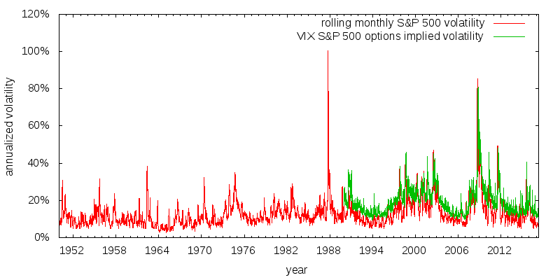
The Black-Scholes model can be used in reverse; to determine the implied volatility given an option's price. The VIX volatility index shows the volatility implied by the price of close-to-the-money S&P 500 index options.
Data for the VIX index is available since 1990. Figure 1 plots the realized historical volatility of the S&P 500, along with the value of the VIX. Several things are apparent. First, the realized volatility shows no discernible trends from 1950 to the present day. This is useful, as it means we can readily use past results for making future volatility predictions. Second, the VIX consistently over-estimates realized volatility. This is not so good; it means we will consistently overpay when purchasing options. Overpaying wouldn't matter so much if we were actively trading options. What we lose when buying we gain when selling. But because we plan to hold options for an extended period this over-pricing could be a real problem.
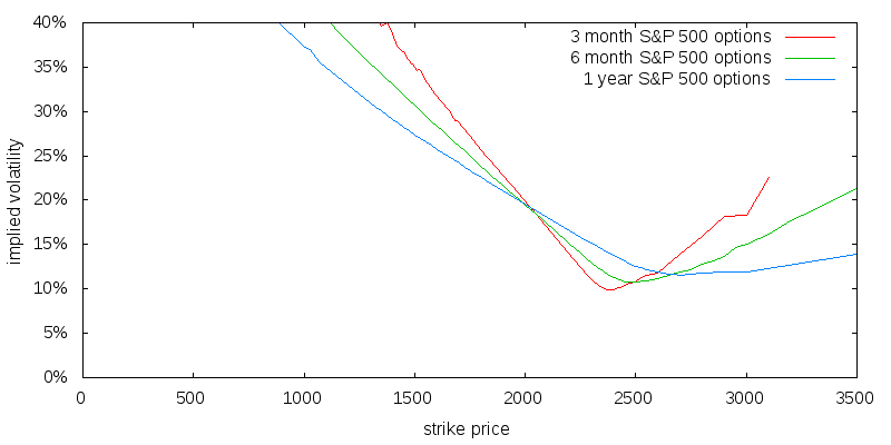
In a perfect world implied volatility would be independent of strike price and equal to the true expectation of market volatility. The world is not perfect however, and plotting implied volatility as a function of strike price reveals a strong pattern, as shown in Figure 2. The overall shape is referred to as a volatility smile, and the slope is referred to as volatility skew. Not only are close to-the-money option prices inflated because the VIX over-estimates volatility, but the price of in-the-money call options is further over-estimated because of volatility skew.
Implied volatility is computed assuming put-call parity, a technical relationship between the price of a call and a put at the same strike price assuming no arbitrage conditions exist. Under put-call parity the implied volatility of puts and calls is identical. The parameter that gets tweaked to ensure put-call parity is the index's forward price, or equivalently implied dividends. These implied values may differ from the true expected values.
The map of implied volatility as a function of strike price and option duration is known as a volatility surface. The volatility surface may evolve over time.
One interpretation of volatility skew is the market is pricing the consequences of a fat-tailed return distribution, which includes extreme negative events, and as a result boosting the price of deep in-the-money put options, and thus their associated implied volatilities. As a consequence of put-call parity this also boosts the equal implied volatility of call options. Under this interpretation of volatility skew it would be unfair to compute the fair price of the call option using a simple expectation of future volatility. Instead this expectation of future volatility should be scaled up by a factor equal to the ratio of the observed implied volatility for the strike price to the observed at-the-money implied volatility.
From 2012 through 2016 volatility has been relatively stable with a mean value of 12.9% when computed in daily log terms. Using the Black-Scholes equation, the appropriately scaled volatility over the previous year as my expectation of future volatility, and an expectation of future dividends equal to the end of year trailing twelve month dividend yield, enables me to calculate the projected fair price of a call option as a function of strike price. Comparing the difference between the quoted price and the computed fair price enables the computation of the call price premium, which is the amount paid above the fair price. This is shown in Figure 3. Quotes were taken at 3:45pm on 2016-12-19, rather than at the 4:00pm market close, as the market is considered to be more liquid at the earlier time.
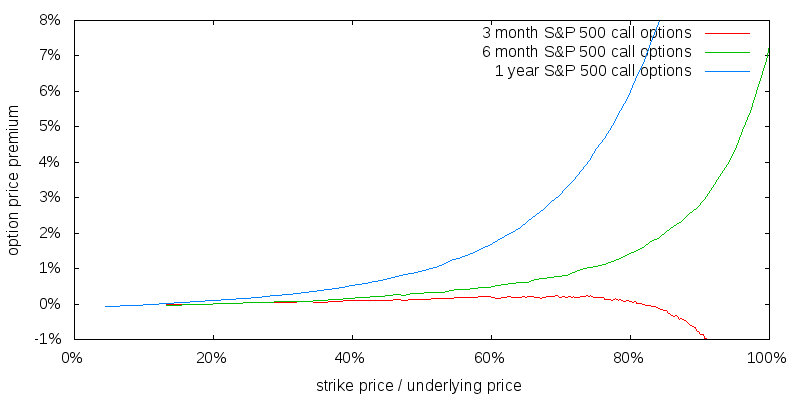
The pricing of close to-the-money shorter duration call options is very sensitive to expected future volatility. Using an expected future volatility value that is 1% less than that of the previous twelve months' value results in an upward slopping option price premium for all three durations. The price premiums of deep in-the-money call options are relatively constant.
There are two ways we can keep the price premium of call options low: purchasing them with low strike prices, or by keeping their duration short.
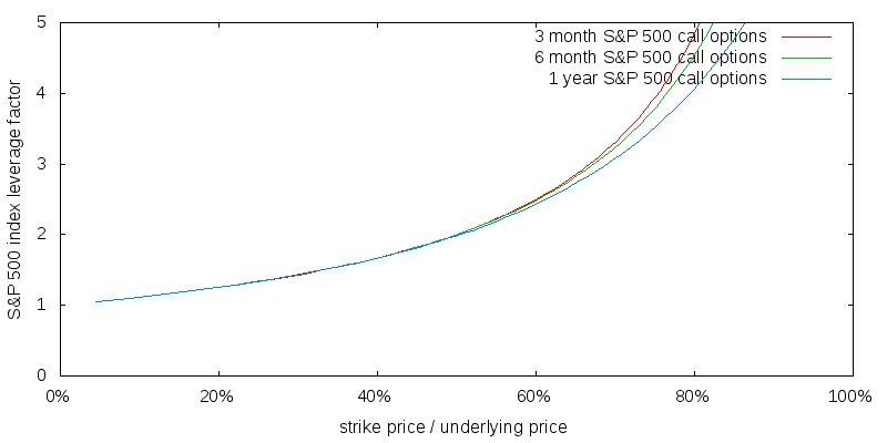
I am interested in the leverage available from purchasing call options. The amount of leverage obtained is equal to the current index price divided by the quoted price of the call option. To which I apply a multiplicative adjustment factor known as delta which reflects the change in price of the call option as a function of change in price of the underlying index. Delta is obtained by differentiating the Black-Scholes equation with respect to the index price. Figure 4 illustrates the projected amount of leverage obtained over the S&P 500 index from call options as a function of strike price.
In Effective Altruism Asset Allocation I suggest a reasonable model of utility for an individual is a constant relative risk aversion (CRRA) utility function with a coefficient of relative risk aversion of 2. However things become more complicated for an effective altruist because only a fraction of consumption is likely to be correlated with the returns of the optimal level of market leverage, while the rest can be treated as uncorrelated. As it turns out the exact coefficient of relative risk aversion, and the exact amount of correlated assets doesn't matter greatly. What matters most is the is some uncorrelated consumption that acts as a brake on the worst aspects of a CRRA utility function at small levels of consumption. As a result of this a reasonable asset allocation for effective altruism portfolios is probably around 300% stocks.
The S&P 500 index is nominal, and does not include any dividends received. As a result the leverage in total return, which is what we care about, will be slightly less than the leverage on the index. In general:
For instance an index leverage factor of 3.3 corresponds to a total return leverage factor of 3.0; assuming an arithmetic mean annualized real stock market return, R, of 4.5% (this value is justified in Effective Altruism Investing Strategies), a 2.3% inflation rate (based on the Survey of Professional Forecasters April 2017 inflation projection for 2017), and a 2.0% dividend yield (S&P 500 dividend yield as of April 2017):
For 1-year call options a leverage factor of 3.3 corresponds to a strike price of 73% of the underlying price. Thus we should buy call options at this strike price. The next question becomes how expensive are call options with this strike price relative to their fair price.
Per the earlier figure, 1-year call options with a strike price of 73% have a price premium of 3.8%. This premium is simply too large for the 300% leverage that would be gained. In Effective Altruism Investing Strategies: Leveraged ETFs I found there that without any penalty a 300% stocks portfolio was 130% better for effective altruism purposes 100% stocks, but that with a 1.8% per annum performance penalty a 300% stocks investment was only 30% better than investing in 100% stocks with a 0.1% performance penalty (where better is loosely interpreted as the ratio of certainty equivalent donation amounts). In any case a 3.8% penalty would be far from being able to compensate for the increased risks associated with the 3X increase in volatility.
The option price premium on 6-month options providing 300% leverage is 0.8%, which is a big improvement, but it will have to be paid twice along with any spreads. And 3-month options look even more attractive.
The spread is the difference between the bid and the ask price. By convention, analysis is usually performed at the mid-point price. In addition to the price premium it would be necessary to pay perhaps half the call spread when entering a position, and again if leaving a position. Figure 5 shows the call spread as a function of strike price.
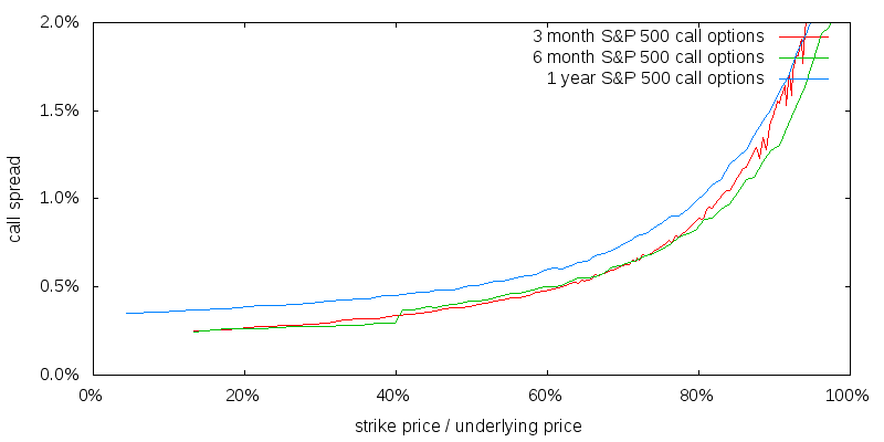
Although shorter duration call options are more attractive from a price premium perspective, they are less attractive from a spread basis because the spread will have to be paid several times per year as the options are rolled over.
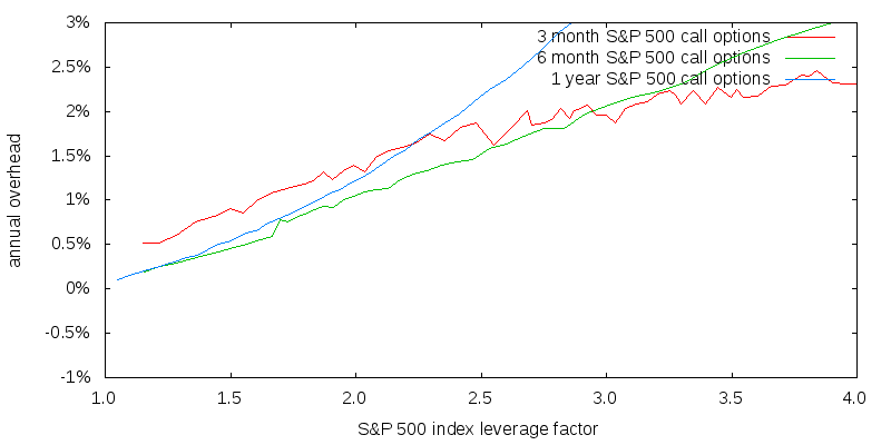
Figure 6 shows the total annual overhead (price premium plus half spread) associated with purchasing call options of different durations as a function of the index leverage factor. The cost of the spread largely eliminates the advantage of shorter duration options.
The volatility surface changes over time. We are less concerned about evolution of the volatility surface per se, and more concerned with how its evolution may affect the annual overhead cost as a function of the S&P 500 leverage factor for a given deep-in-the-money strike price.
I computed the annual 1-year call option overhead cost every December of 2004-2016 as shown in Figure 7. The different lines are a result of both the evolution of the volatility surface, and differences in the estimates of expected future dividend yields and expected future volatilities.
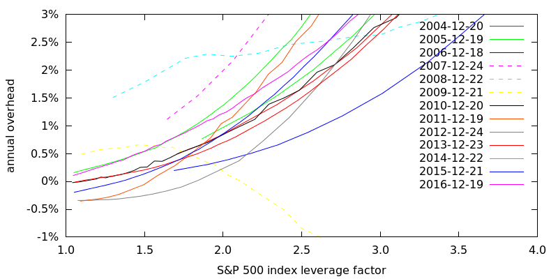
A majority of the lines are bunched together over a reasonably small range. That they differ is both because the volatility surface evolves over time and because trailing twelve month dividend yields and 1-year prior volatilities did a poor job of representing reasonable future expectations. The 3 most widely divergent lines were for 2007-2009, around the time of the subprime mortgage crisis, when 1-year prior volatilities most likely did a poor job of representing expected future volatilities. Sometimes using past historical values for future expectations will produce an overestimate and sometimes an underestimate, but since dividend yields and volatilities don't show any significant trends over the period of analysis this won't introduce any systematic bias in the results.
Figure 8 shows the average overhead for 2004-2016 for different option durations with 2007-2009 excluded. I removed 2007-2009 because expected future volatilities were then poorly predicted by past volatilities reducing the accuracy of the data. Including them would, as it happens, not have significantly altered the projected average annual overheads. In each case expected dividends were trailing twelve month values for that month and expected volatilities were those of the prior 12 months.
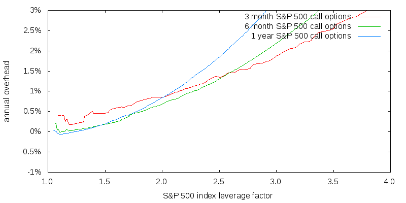
As the target index leverage factor increases the duration of the best performing call options decreases.
I developed an asset allocator called Opal that uses stochastic dynamic programming to determine the optimal asset allocation and donation strategy as a function of age and portfolio size. Opal can also be run in non-stochastic dynamic programming mode to compute the certainty equivalent utility associated with a given initial portfolio size, fixed asset allocation, and fixed donation strategy. A certainty equivalent is the constant annual donation amount that has the same utility as the probability weighted set of all possible variable donation sequences that might be experienced. Table 1 presents the certainty equivalent donation amounts for a sampling of the expected best performing call options. The use of a 50 year period is so that a majority of the donation amount is made from from investment returns, not the original principal, thus maximizing the difference between the strategies.
| call option duration | mean strike / underlying price | index leverage | estimated total return leverage | annual overhead | annual certainty equivalent donation amount | |
|---|---|---|---|---|---|---|
| without overhead | with overhead | |||||
| 100% stocks | 0.1% | $12,008 | $11,691 | |||
| 1 year | 33% | 1.5 | 1.09 | 0.2% | $12,778 | $12,132 |
| 6 months | 33% | 1.5 | 1.09 | 0.2% | $12,840 | $12,186 |
| 6 months | 50% | 2.0 | 1.62 | 0.7% | $17,711 | $15,135 |
| 6 months | 61% | 2.5 | 2.16 | 1.3% | $20,323 | $15,816 |
| 3 months | 60% | 2.5 | 2.16 | 1.3% | $20,666 | $16,105 |
| 3 months | 67% | 3.0 | 2.69 | 1.9% | $20,714 | $15,043 |
| 3 months | 72% | 3.5 | 3.22 | 2.6% | $18,813 | $12,726 |
| 100% small cap value (no anomaly) | 0.1% | $17,479 | $17,060 | |||
| 100% small cap value (anomaly) | 0.1% | $41,009 | $40,177 | |||
Looking at the different call options, 3-month call options with a strike price equal to 60% of the underlying price have the best expected performance, and, once the annual overhead is factored in, provide a certainty equivalent donation amount that is 38% above that for 100% large cap stocks.
The table also shows the expected performance of a 100% (large cap) stock and 100% small cap value strategies. The performance of all deep in-the-money call option strategies is inferior to the expected performance of small cap value stocks. This is true if small cap value is evaluated on a purely risk adjusted basis (no anomaly), and more so if there is a future 4% small and value performance anomaly as there has been in the past (anomaly).
Purchasing 3-month deep in-the-money call options and rolling them over four times a year offers a significant expected performance improvement over investing in 100% stocks. However, the complexity of this approach, including the possible need to rebalance in the event of a very large downturn, and that it appears inferior to simply investing in small cap value means I wouldn't recommend it.
Data was sourced from Yahoo Finance and CBOE. CBOE data files cost $6.54. Data was analyzed using a 600 line Python program called Stock Options Analyze. Data was plotted using the stock_options.gnuplot GnuPlot script.
© 2017 Gordon Irlam. Some rights reserved.
 This work is licensed under a Creative Commons Attribution-ShareAlike 4.0 International License.