A reasonable rough estimate of the coefficient of relative risk aversion of consumption is in the range 1-4. It is estimated that 10-40% of cause consumption is correlated with the optimal effective altruism investing strategies. And finally effective altruists may wish to discount future utility at a rate of 0-10%. Taken together this suggests that in an ideal mathematical world effective altruists should adopt heavily leveraged stock portfolios comprising roughly 300% stocks. I discuss the many practical difficulties associated with this recommendation elsewhere. The gains that might be realized from such an allocation if it is obtainable are in the range of 3-fold relative to 100% stocks. Even a small amount of donations that are uncorrelated with the optimal investment strategy are found sufficient to drastically increase recommended asset allocations beyond those computed using the Kelly criteria or Merton's portfolio problem solution.
This article expands on Effective Altruism Investing Strategies by exploring reasonable theoretical asset allocations for effective altruism portfolios.
Risk aversion is the desire to reduce uncertainty in investment outcomes. Determining the appropriate degree of risk aversion associated with effective altruism causes is fundamental to effective altruism investing. A low degree of risk aversion implies taking your chances on a highly leveraged stock portfolio, while a high degree of risk aversion implies holdings of cash or other stable assets.
Utility is a concept from economics that expresses the amount of satisfaction received or good done by a particular amount of consumption or donations. Suppose the total amount of good done at time t by consumption C is ut(C).
Implicitly here I am assuming the ut are independent of each other with respect to time. This means:
It is common to model utility using what is known as a Constant Relative Risk Aversion (CRRA) utility function:
where C is the consumption, and γ is termed the coefficient of relative risk aversion.
A γ of 0 corresponds to risk-neutrality; indifference to risk, and implies unlimited exposure to risky assets, and optimizing for the arithmetic mean return. A γ of 1 indicates logarithmic utility and implies asset allocation using the Kelly criterion. A γ greater than 1 denotes increasingly strong risk aversion.
The Kelly criterion is a special case of the more general Merton's portfolio problem which provides the appropriate asset allocation for an arbitrary value of γ.
In general the coefficient of relative risk aversion with respect to consumption C is defined as:
When the coefficient of relative risk aversion is a constant, γ, the utility function is a unique CRRA utility function, apart from scaling and constant of integration.
From the definition of CRRA utility, we see that marginal utility, that is the incremental good from an incremental dollar is,
To get a feel for this Table 1 shows some possible values of γ and the relative marginal utility when the donation amount is halved or doubled.
| γ | relative marginal utility | |
|---|---|---|
| halve C | double C | |
| 0.4 | 132% | 76% |
| 0.6 | 152% | 66% |
| 0.8 | 174% | 57% |
| 1.0 | 200% | 50% |
| 1.5 | 283% | 35% |
| 2.0 | 400% | 25% |
| 4.0 | 1,600% | 6% |
A value for γ of 1.0 says that the impact of a marginal dollar at donation level C/2 is 200%, or double, that of a marginal dollar at level C.
For individuals a coefficient of relative risk aversion of 1 to 4 is probably reasonable. This is a big range. Studies of how people behave in response to risks tend to support a value around 1, while surveys of how people feel about risk and how they invest tend to support a value of 4 or even higher. My best guess estimate for the value of γ for most individuals is 2. I find the high end of these estimates implausible in view of the results presented in Table 1. I discuss the broad range of uncertainty regarding an appropriate coefficient of relative risk aversion for personal investing elsewhere.
For a CRRA utility function the solution to Merton's portfolio problem can be used to estimate the proportion of stocks, π, that should be held by an investor, with the remainder held in risk free cash:
where RWeiner is drift of the Weiner process generating the return of stocks, σWeiner its standard deviation, Rrf,Weiner is the drift associated risk free rate, that is, the drift on short term Treasuries, and γ is the coefficient of relative risk aversion. These values may be computed from R, the arithmetic mean annual return of stocks, σ its standard deviation, and Rrf, the risk free rate, that is, the annual return on short term Treasuries, as:
Great care must be taken in applying Merton's solution since it is only applicable to a CRRA utility function. The optimal stock holdings for a non-CRRA utility function lacks an analytical solution. To compute the optimal stock holdings in this latter case it is necessary to solve Merton's equations numerically. This requires the use of stochastic dynamic programming, which solves the problem by working back from the oldest age to the youngest.
Using our estimate of γ and plugging in some numbers representative of the U.S. stock market over the period 1970-2016 gives:
In other words, in the absence of uncorrelated consumption, you should probably borrow at the risk free rate in order to secure a slightly leveraged position in stocks.
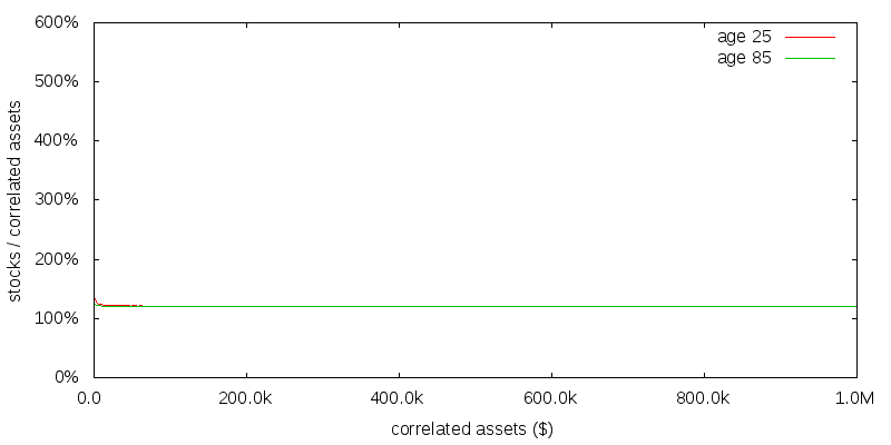
Figure 1 shows the numerical solution to this problem computed using stochastic dynamic programming. This figure is in good agreement with the theoretical prediction. The lines for age 25 and 85 are almost totally coincident, with an optimal strategy of 121% stocks independent of age and correlated assets amount. Since there is no uncorrelated consumption the correlated asset amount is the same as the total assets held for the cause.
We care about risk aversion because it determines how much to donate and how much investment risk to take. We have to be careful though because in making this determination other investors might share the same investment strategy as us, making investments correlated. A simple model of C then is:
In which C has been split into donations and other amounts that are uncorrelated and correlated with our donation amount. The correlated donations magnify our donation, Cdonate by a factor of K:
For many effective altruism causes there is reason to believe that Ccorr is quite small in comparison to C.
Based on these considerations a reasonable value for Ccorr might be 10-40% of C, with a best guess estimate of 25%.
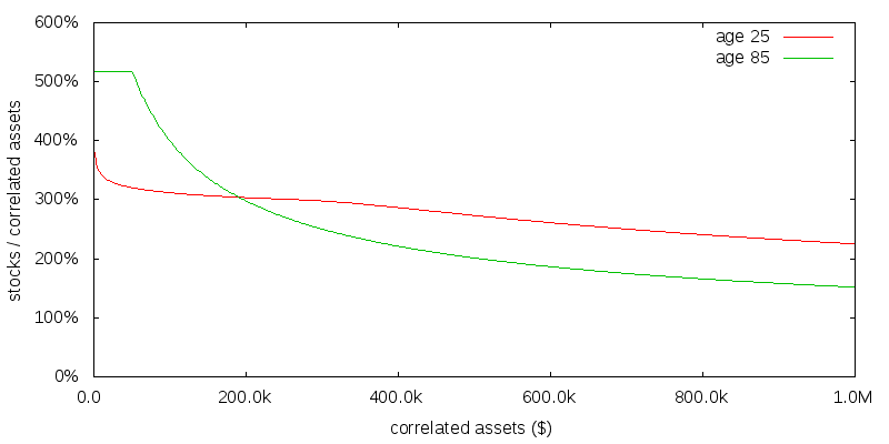
Figure 2 shows the optimal strategy computed numerically in the presence of uncorrelated assets providing $100k per year of consumption. Not only have the correlated asset allocations increased significantly across the board, but they are no longer constant as a function of age or correlated assets size. If 10% is a reasonable average donation rate for the correlated assets (the true amount will vary as determined by stochastic dynamic programming), and 25% is a reasonable value for Ccorr / C, then $330k would be a reasonable value for the correlated assets.
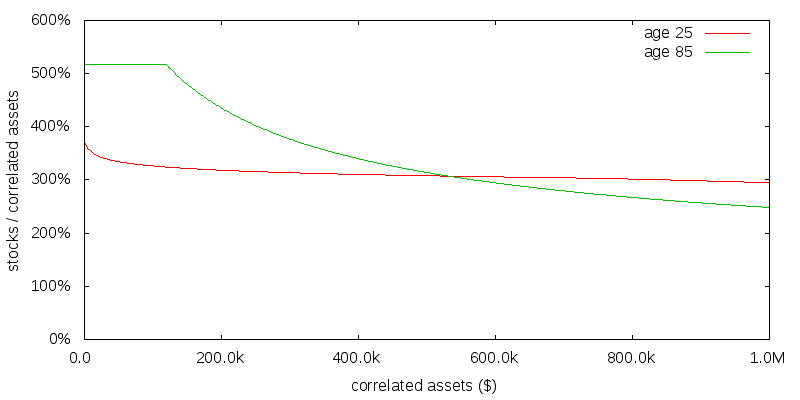
The capping of the recommended allocation to stocks at about 520% is an artifact of rebalancing being performed on a monthly basis. At a higher allocation than this with monthly rebalancing there was the possibility of the portfolio becoming negative. If rebalancing was performed continuously no such limit would exist.
How do we reconcile the very different asset allocation results with and without uncorrelated consumption? No uncorrelated consumption is the same as saying Ccorr / C is 100%, pushing Ccorr to infinity. We thus have to extrapolate the far right of the previous figure at which point the figure is presumed to coincide with the no uncorrelated consumption case. This convergence can be seen more clearly in the graph for uncorrelated consumption sensitivity presented later.
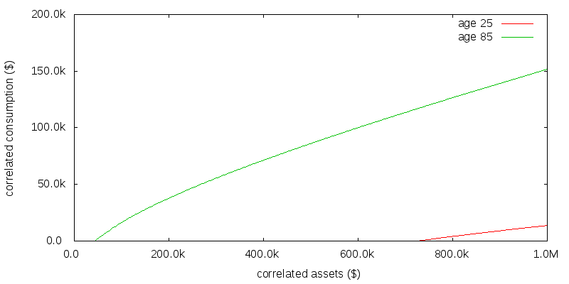
Figure 3 shows the correlated consumption amount as a function of correlated assets. Unlike Merton's portfolio problem, in which the optimal solution is to consume a fixed proportion of wealth as a function of age, the optimal strategy now is not to consume any correlated assets until a given age-dependent correlated asset size is reached.
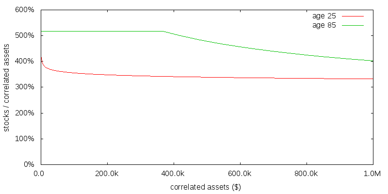
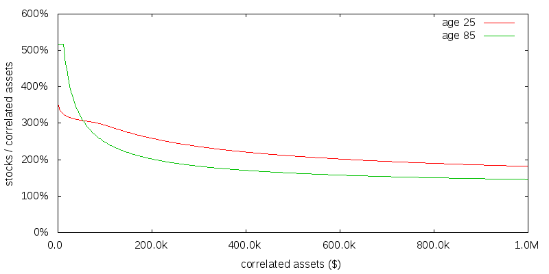
Figures 4 and 5 repeat the previous exercise for a γ of 1 and the slightly less plausible value of 4. For a reasonably young effective altruist the optimal asset allocation seems relatively insensitive to the precise coefficient of relative risk aversion. Based on all of these figures the optimal asset allocation for effective altruism portfolios is probably somewhere in the range 300-360% stocks for a reasonably young effective altruist in the absence of time discounting.
I have been assuming $100,000 of uncorrelated consumption per year. Figure 6 shows the effect of reducing this to $10,000. As might be expected this has the effect of shrinking the graph along the x-axis.
Even a small amount of uncorrelated consumption is sufficient to substantialy increase the optimal asset allocation above that of the no uncorelated consumption case.
The value of future action may be less than present action for a variety of reasons. Figure 7 presents the effect of applying a 10% annual discount rate to utility in the $100k per year of uncorrelated consumption, γ=2, scenario. This is considered a high degree of time discounting. The result is to increase the stock allocation for small amounts of correlated assets at age 25, but leave it largely unchanged for large amounts of correlated assets or at age 85.
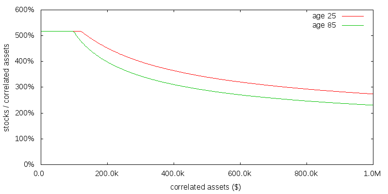
Based on this and the previous results, the optimal asset allocation for a reasonably young effective altruist, with no to moderate time discounting, is probably in the range 300-400% stocks. For older effective altruists similar conclusions would likely apply provided utility was still considered to be obtained from any remaining assets after death; a simplification made in this numerical model was that there is no value associated with donating assets after you die.
So far we have been considering the optimal asset allocation as a function of age and correlated assets size. How might a simpler fixed asset allocation compare to the optimal asset allocation? The concept of certainty equivalence helps us answer this question.
The certainty equivalent is the constant annual donation amount we would be indifferent to making in comparison to the unknown sequence of donations we expect to make as by adopting some strategy in the presence of the stochastic market returns. I won't go in to the details, but suffice to say for a given utility function it is possible to compute certainty equivalent values for different asset allocation and donation strategies.
Table 2 shows the certainty equivalent donation amount for various asset allocation strategies. This table shouldn't be taken as gospel, but should be seen as indicative of the sorts of gains that might be possible through the use of leveraged positions. Adopting a leveraged position can boost the effective donation amount by more than a factor of 3. This is huge. Also note a 300% stocks asset allocation does almost as well as the optimal variable strategy.
| asset allocation | annual certainty equivalent donation amount |
|---|---|
| 100% stocks | $12,875 |
| 100% small cap value | $19,929 |
| 200% stocks | $32,683 |
| 300% stocks | $37,829 |
| 400% stocks | $30,728 |
| optimal dynamic stocks | $41,861 |
Important reasons Table 2 might not be applicable include:
These computations were performed on a monthly, not an annual basis. If rebalancing was only performed once per year, there is greater risk for a leveraged portfolio to becoming negative, limiting the maximum amount of leverage that would be recommended, and the resulting upside.
A legitimate criticism of these results is they were performed with a fixed uncorrelated consumption amount, rather than a stochastically variable but uncorrelated consumption amount. The stochastic dynamic programming approach lends itself to determining the optimal strategy in the presence of a stochastically variable uncorrelated consumption amount, albeit at the expense of an additional month or so of programming effort, and considerable additional compute time. This appears a fruitful area for additional research.
To avoid problems calculating with infinities the numerical no correlated assets case was actually computed with $1 per year of uncorrelated consumption.
Life expectancy was modeled stochastically using a Gompertz distribution with a total life expectancy at age 25 of 83 years.
© 2016-2017 Gordon Irlam. Some rights reserved.
 This work is licensed under a Creative Commons Attribution-ShareAlike 4.0 International License.