A spending strategy specifies how donations will evolve as a function of time, wealth, and donation history. Spending strategies appear only moderately important. Depending upon the cause, the gains from the optimal spending strategy compared to spending at a constant rate were found to be in the range 19% to 29%.
Stochastic dynamic programming is a powerful technique for precisely determining spending strategies. Unfortunately its power is limited by the accuracy with which it is possible to determine the discount rate associated with causes.
Delay spending while knowledge is still being gained. The rate of knowledge gain by the effective altruism community is impressive, and it implies delaying making major donations. Give early to high discount rate causes. You should give early to causes with a discount rate that exceeds the arithmetic mean investment rate of return. Give late to low discount rate causes. Unfortunately discount rates are often difficult to determine. The optimal strategy is almost always peaked and almost never to give a constant amount over time. However, depending on the discount rate, donating a constant amount over time may incur a relatively small cost.
Personal satisfaction can be invoked to explain donating over an extended period, but since money grows over time and satisfaction does not get discounted it will favor donating during later ages.
Mean and median spending plans diverge significantly. Mean spending includes a small number of massive outliers where the market returns did very well boosting the mean significantly.
Estate plans don't greatly alter spending plans. The efficiency with which you leave money to causes through your estate has a relatively small effect on spending strategies.
Experience counts for little. Optimal spending strategies don't seem to be greatly perturbed when you factor in the need to make donations in order to find out what works best.
Investment strategies appear more important than spending strategies. A small cap value investment strategy was found to increase impact by anywhere from 29% to 101% relative to a 60/40 stocks/bonds investment strategy.
Effective altruism is a movement that seeks to use reason to achieve the most good in the world. This article deals with when and how much to donate.
Being an earn-to-give effective altruist requires paying attention to four factors:
Deciding whether and how much money to spend now, versus allowing it to compound, and spend more later is a decision faced by all effective altruists. Three common spending strategies are spend now, spend later, and spend a constant amount over time. These are not the only strategies possible, and in general a spending strategy will be a function of time, wealth, and if spending experience matters, the prior spending history.
Throughout this paper I usually assume lognormally distributed real annual investment returns with an arithmetic mean of 6.5% and a standard deviation, or volatility, of 22.2%. This corresponds to a geometric return of 4.3% and is considered indicative of the expected returns for small cap value stocks going forward. Occasionally I also explore the effects of a sub-optimal investment strategy, for which I use returns with a real arithmetic mean of 2.9% and a volatility of 10.5%. This corresponds to a geometric return of 2.4% and is considered indicative of the returns for a 60/40 stock/bond portfolio going forward. By historical standards these are low return expectations, but this is the result of the low interest rate environment we are now in, and which is largely expected to persist. Further details on how these values were chosen are given elsewhere.
I also assume an individual age 25 with an initial wealth earmarked for effective altruism causes of $200k, and no additional contributions made. No additional contributions made is for pedagogical simplicity. A complex contribution pattern can always be mapped back to an equivalent initial wealth unless there is a wealth constraint violation, in which case donations would need to be delayed. The exact initial wealth doesn't matter greatly. I chose $200k because it is roughly equivalent to having $1m for effective altruism causes at age 65, assuming a 4.3% geometric rate of return. Achieving $1m would require contributing $10k every year. $10k per year is doable. As a point of comparison $10k is what is required to build a $600-700k retirement nest egg assuming constant contributions and a more risk averse 2.4% geometric rate of return.
Critical to the spending decision is the idea that early money is usually more valuable than late money. This is captured by the mathematical notion of a discount rate. A 3% annual inflation adjusted discount rate means that $1 donated today is as valuable as an inflation adjusted $1.03 donated in a year's time. Throughout this paper all amounts and discount rates are given in real, inflation adjusted, terms.
Discount rates vary for both objective and subjective reasons. An objective reason is it will be harder to achieve the same result in a year's time. A subjective reason is we might value the future less than we do the present.
Discount rates differ both across causes and over time. For instance there is a sweet spot for funding smarter-than-human AI risk mitigation when funding will do the most good. Too early, and funding is unlikely to have an impact, and too late and the problem will likely be too big to do much about. Very early on the discount rate would have been negative, indicating that late money would more valuable than early money. Over time the discount rate might rise to zero. The point at which the discount rate is zero is the point of maximum fiscal impact. Beyond this point the discount rate will be positive, indicating that earlier money is more valuable than later money. For contrast animal welfare is likely to have a small positive constant discount rate. I use r(t) for the discount rate at time t.
In the previous paragraph I said the point of maximum fiscal impact is when the discount rate equals zero. This is true only if no investment is occurring. If the arithmetic rate of investment return is R, then assuming linear utility (as discussed later) the point of maximum fiscal impact will be when r(t) = R. If r(t) is always less than R, then this means we can always do more expected good by delaying for a year, and investing the money, than we could do spending the money today.
For the mathematically curious, if Ut(C) is the amount of good done by C dollars at time t, then the r(t) is
Where dX/dt denotes the derivative of X with respect to time t.
Individual causes have discount rates. There also exists an overall discount rate across all causes. It could be computed as r*(t) based on
At any one point in time a single cause is likely to take on the maximum value and thus determine the discount rate. This means the overall discount rate will be varying over time, not just because it slowly varies over time within a cause, but abruptly because the top cause changes. The resulting uncertainty over the discount rate makes determining the optimal strategy very difficult. Over a long enough time discount rates are likely to average out to something close to the growth rate in the overall economy. If they did not you could point either forwards or back to a time when there exists a particular cause that is arbitrarily many times larger than the economy.
Throughout this paper I start with discount rates that are constant over time. Not because discount rates don't vary over time, but because it is hard enough to determine the correct discount rate, let alone specify how it varies over time. It is important to stay alert to the dangers of this simplification.
Here are some example discount rates to consider:
The effective altruism movement is in its early days, meaning that new causes with better payoffs than existing causes might yet to be uncovered, or a more thorough analysis might show the superiority of one particular neglected cause. When this happens there could be an abrupt one time blip in the discount rate of -50%, or even more negative. I choose to model this as a separate knowledge factor that multiplies things by a constant amount that is increasing over time. This breaks the problem down into two components. What is a reasonable knowledge factor to use? And what is a reasonable underlying constant discount rate?
Utility is a concept from economics that expresses the amount of satisfaction received or good done by a particular amount of consumption or a donation.
Let ut(C) be the utility obtained from consumption C in time period t, and let Ut(W) be the utility obtained from the scheduled consumption of wealth W over period t and all subsequent periods. For an arbitrary utility function, ut(C), constructing the optimal spending strategy as a function of time and wealth so as to maximize U0(C) might at first seem like a difficult problem. How much should we spend today, when the amount we spend today will influence the amount we can spend tomorrow? And the amount we spend tomorrow will influence the amount we can spend the day after.
Suppose we have a fixed rate of return, g. The problem can then be solved if we work backwards. Let Ct(Wt) denote the optimal consumption at time t for wealth Wt. In the final year we should donate everything, and obtain a utility UT(WT) = uT(CT(WT)). Since WT is currently unknown, we have to compute this utility for each possible value of WT. Since this is the final year CT(WT) = WT. With this in hand we can then proceed to the prior year, and for each possible value of WT-1, we can compute the consumption CT-1(WT-1) that maximizes UT-1(WT-1) according to the following equation,
The future period utility term in the utility sum can be looked up from the values we have previously computed. In both terms, CT-1(WT-1) is unknown, but we can compute it by trial and error to maximize the utility sum. We do this for each possible value of WT-1. Then we proceed to T-2 using the values we have computed for T-1, and so on, until we reach T=0. We then have the optimal consumption strategy Ct(Wt) where Wt follows the wealth equation,
and W0 is known.
This is dynamic programming in its simplest form. It assumes a fixed rate of return, which isn't realistic.
In stochastic dynamic programming the rate of return is variable, and instead of a single growth rate, you choose a representative bundle of growth rates, the wealth equation yields a set of wealth equations, and the future period utility term in the utility sum is replaced by the weighted mean value of a set of such terms.
I determine an optimal strategy that takes into account improved utility based on past spending experience. To do this I compute things based on the amount spent in the last period, in addition to computing things based on each possible wealth level. This turns ut into ut(Ct, Ct-1), Ut into Ut(Wt, Ct-1) and Ct into Ct(Wt, Ct-1). This requires additional computational resources, but doesn't present any mathematical difficulties.
I also take into account a stochastic life span by weighting each ut by the probability of being alive at time t.
Stochastic dynamic programming involves performing a trial and error search for each possible wealth level at each possible age. We compute and interpolate on a grid. For this we might need 500 wealth levels, 500 spending levels, and roughly 80 ages. If each trial and error search involves evaluating the total utility at perhaps 10 different consumption values, and we use a bundle of 10 representative growth rates, then we have to lookup the future utility 2 billion times. This is a non-trivial amount of computing, and takes around 10 minutes on a single core of a 2015 vintage computer.
I implemented the stochastic dynamic programming approach to the spending strategy problem in a 1,200 line Python program called EA Spend. For performance reasons it should normally be run using the PyPy just-in-time Python compiler.
The program also generates 100,000 random return sequences. Starting with the initial wealth level the program computes how each return sequence performs employing the optimal strategy. This makes it possible to compute mean, median, and percentile donation levels as a function of age.
Utility conflates two concepts. Risk aversion: how we feel about different possible outcomes. And intertemporal substitution: how we feel about donating now versus later. Epstein-Zin preferences separate these two concepts, allowing us to express how we feel about risk separately from intertemporal substitution.
Stochastic dynamic programming is fully compatible with using Epstein-Zin preferences. I avoid using Epstein-Zin preferences only because it is hard enough to specify a single value for risk aversion and intertemporal substitution. Having two separate parameters that have been specified would only complicate interpreting the results. Nonetheless, Epstein-Zin preferences are a promising area for future work.
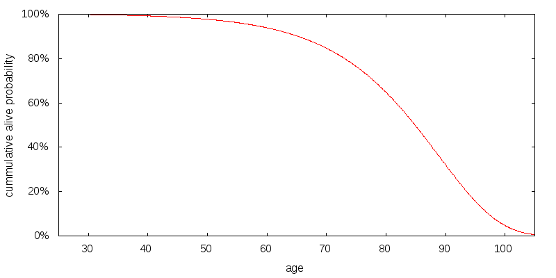
I considered a 25-year-old with a total life expectancy of 83 years. I constructed a Gompertz distribution to match this life expectancy. The resulting probability of being alive as a function of age is shown in Figure 1.
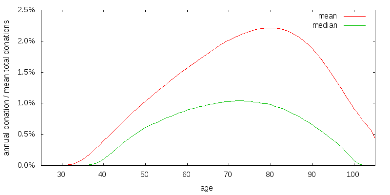
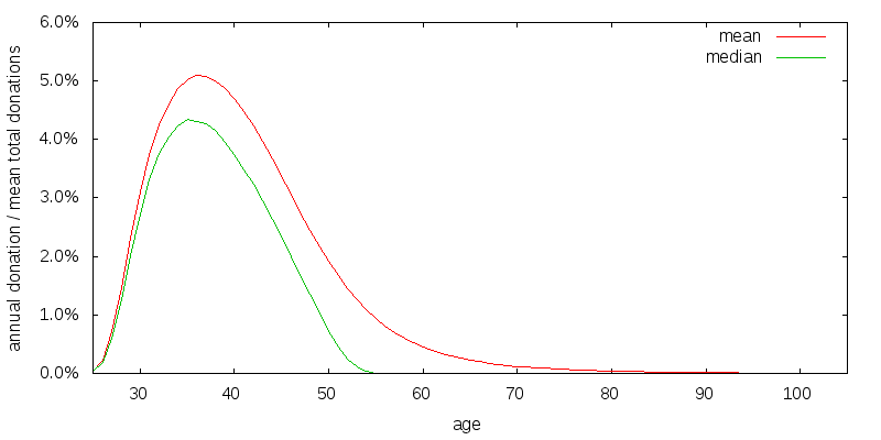
Figure 2 shows the optimal spending strategy for the simplest of scenarios, one in which all utility is derived from donations. I consider a scenario in which there is $100k of uncorrelated donations per year, and the coefficient of relative risk aversion of consumption is 2.
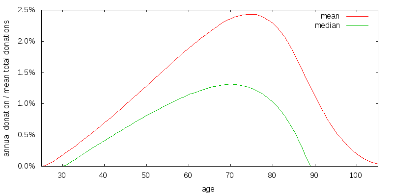
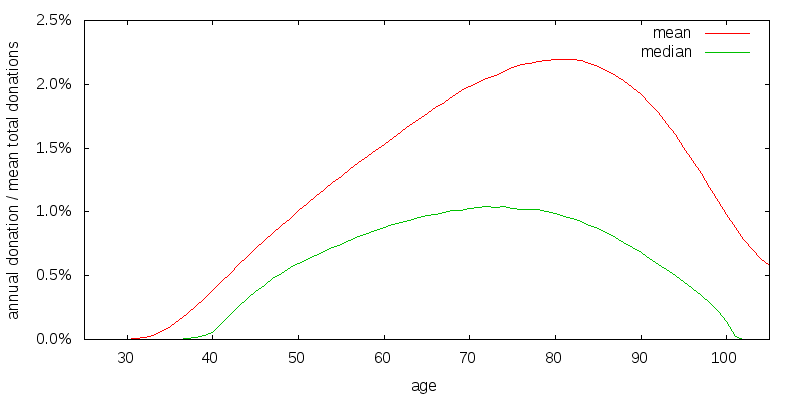
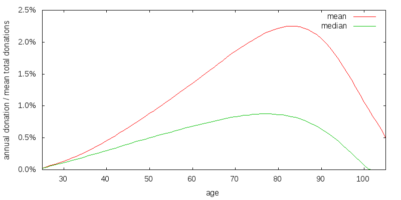
A spending strategy is strictly speaking a function of age and wealth (as well as potentially the previous donation amount). This is difficult to present graphically. What I do instead is construct a number of stochastic return sequences, compute the spending path for each return sequence, and then present the mean and median spending amounts for each age associated with these spending paths. The spending amounts are scaled so that the mean of the total of each donation path over all ages equals 100%. The optimal strategy is to allow your money to compound, and gradually increase your donations, until you are in your 70's, and at least in the median case to have donated it all by age 89. The median donation amount is smaller than the mean donation amount. The utility discount rate is 3%, and the investment rate of return is 6.5% arithmetic with a 22.2% volatility.
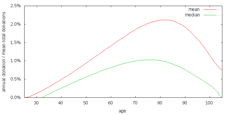
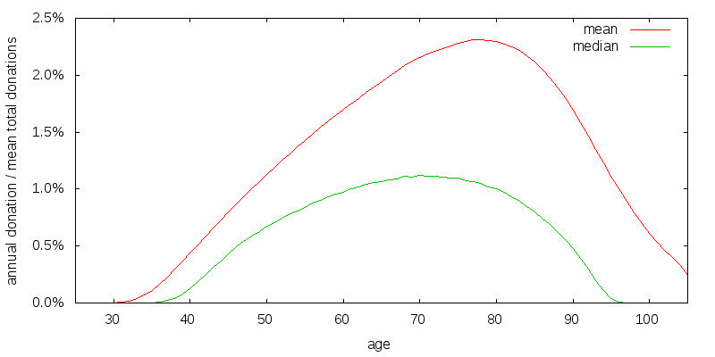
In the previous scenario I implicitly assumed that if you die your money goes to waste. This is probably not true, but it is plausible that money from your estate is spent less effectively than donations made while you are alive. Figure 3 shows the optimal strategy for an estate efficiency factor of 80% of the direct donation efficiency. Utility from direct donations and from your estate are added together to produce total utility. It is assumed that the estate is spent down over 5 years, with the amount spent growing by 30% per year. The optimal strategy involves reducing and delaying the donation amount slightly.
Experience captures the fact that we are more likely to give effectively if we have donated previously. You learn through donating what works and what doesn't, and where money has the most impact. This is especially true for foundations that have to deal with grant agreements on how money will be spent. For large donations there is also the issue of capacity, and recipient organizations can only absorb so much more funding than they received in the prior year. Experience isn't important to all causes, and for some causes experience counts for little.
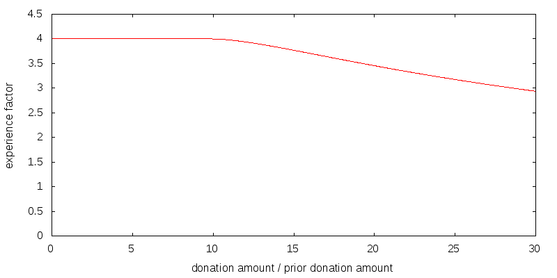
Figure 4 shows my attempt to model a relatively weak experience effect. The overall shape matters, but the details don't. Along the x-axis is the size of this year's donation relative to last year's donation. The y-axis shows the multiplicative factor applied to donation and estate utility. For example, if last year you donated $10,000, and this year you are donating $20,000, you look up the ratio 2 on the x-axis, to get a y-value of 0.93. The $20,000 donation will deliver only 93% of the utility that gets computed before factoring in experience. There has been a loss in utility because the prior $10,000 donation doesn't serve as sufficient experience for a $20,000 donation. In my model a 30% capacity increase each year obtains an experience factor of 1.
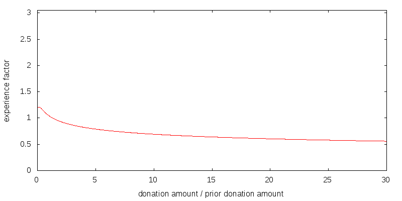
It is important to note that the effects of experience do not compound. Suppose for each of the t previous years you have donated the same amount, for which the experience factor is E(1). Then in year t you will receive E(1) times the base level utility for that amount, not E(1)t times the utility. In my weak experience scenario E(1) has the value 1.04.
Experience effects estate utility in a complex fashion. It is assumed that the estate is spent down over 5 years, with the amount spent growing by 30% per year, and with the previous consumption level for the first year set to zero. Experience factors are computed for each of these five years and applied to the estate utility, which is computed on the annual estate spending amounts. For simplicity, during this process no further investment growth, changes in knowledge, or utility discounting occurs.
Figure 5 shows the optimal strategy when experience matters. It is similar to the estate strategy, although the portfolio is depleted slightly earlier.
Experience captures learning that is dependent on prior donations. I treat this as distinct from learning that is independent of past donations. This latter form of learning is what I describe as knowledge. Knowledge can be because the effective altruism community is finding new causes and better evaluating existing causes. Knowledge can also be because we are new to the effective altruism community and finding out about known causes for the first time.
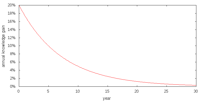
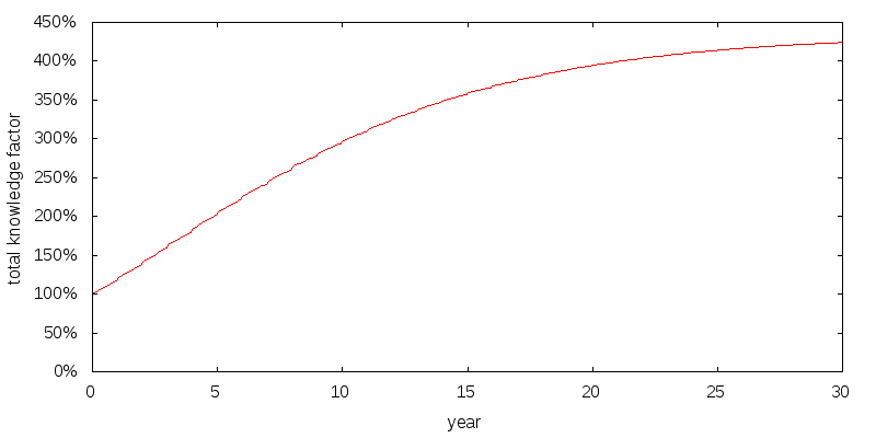
Figure 6 shows how I model a healthy annual gain in knowledge, and Figure 7 shows the resulting cumulative knowledge. Year zero corresponds to age 25. The gains are substantial, and are based on projecting forward the advances of the effective altruism community over the past 10 or so years. After about 15 years the gains flatten off.
Knowledge acts as a multiplying factor applied to the altruism from donations, estate, and experience.
Figure 8 presents the optimal strategy when we add in knowledge. The addition of knowledge delays donations at young ages. The addition of knowledge completes my baseline model. Later I will explore how changes in assumptions effect the baseline strategy.
Depending on the realized market returns the annual donation amount will vary. Figure 9 shows the strategy for baseline model rescaled and with a 95% confidence interval overlaid. The mean donation amount is shown in red. The median donation amount is the small green curve beneath the mean donation amount. And the 95% donation confidence interval is the large green vertical bars. The confidence interval was determined by generating a large number of random market return sequences, computing the donation amounts associated with each sequence, and then determining the 2.5 and 97.5 percentile values. The 95% confidence interval spans an extremely large range. Also note that the upside from the median far exceeds the downside from the median causing the mean to be much larger than the median.
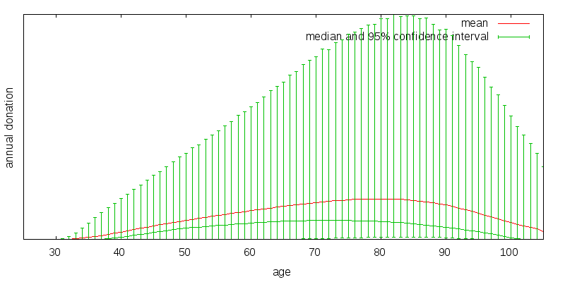
The divergence between mean and median values is a property of all plausible return distributions. For the lognormal distribution the mean value is given by the arithmetic mean compounded over time, while the median value is the geometric mean compounded over time. For instance, the multiplicative difference between the arithmetic and geometric returns in the baseline scenario is 2.1%, which when compounded over 44 years is 2.5. This is comparable to the difference in consumption values for the baseline scenario at age 70, where the median consumption peaks.
This raises the philosophical question: Should effective altruists be seeking to maximize the mean or the median case? The mean is heavily influenced by a few very unlikely scenarios where things go very well. The median is far more likely to occur. It is up to the concepts of utility and risk aversion to capture the extent to which we care about the distribution of donation amounts. The answer to the philosophical question is thus effective altruists should normally be concerned with both, but because of uncorrelated donations should lean more heavily towards optimizing mean utility than the typical investor.
Figure 10 shows the optimal strategy for a geometric and arithmetic mean return equal to the original geometric mean return. This can be thought of as optimizing for the median rather than the mean case. The standard deviation of returns is thus zero, and the mean and median curves are coincident. The curve is similar to median curve presented before. Thus it may not matter greatly which we optimize for.

I will explore the sensitivity of the baseline model constructed previously to the key assumptions made.
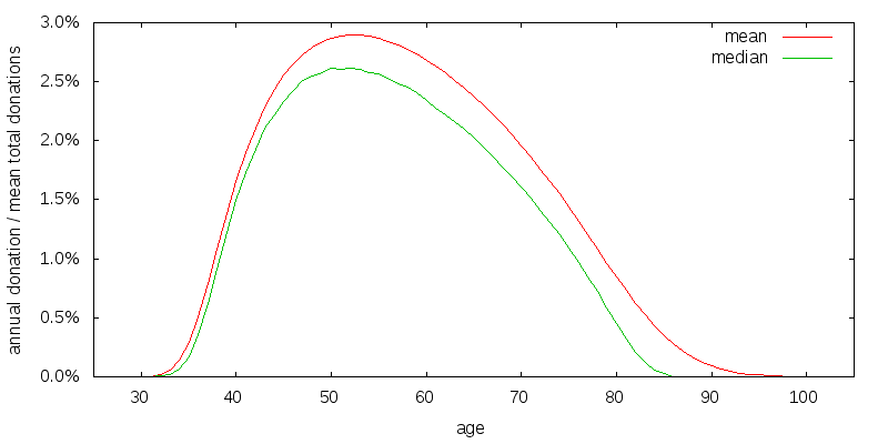
Figure 11 shows the effect of increasing the discount rate for donations, estate, and experience, from 3% to 10%. Early money is now more valuable than late money. This is true even taking into account the possibility of first reinvesting the late money. As expected the curves have been shifted from donating late in life to earlier in life.
Perhaps donating very late in life is a side-effect of the large, 80%, weight I place on estate utility relative to donation utility. Figure 12 shows the effect of reducing estate utility to what I consider a very low value of 50%. Despite this low value the peak of the curves have only shifted left by about 3 years.
What if the gains to experience were greater? Figure 13 shows what I consider to be an extreme experience factor. There is a 4-fold reward for experience, with an ability to increase capacity approximately 10-fold before this 4-fold increase starts to decline. The commonsense requirement that donation utility multiplied by experience factor be a monotone increasing function of donation amount limits how sharply the experience factor falls. If I were not modeling it separately as knowledge, such an experience factor might be appropriate for the effective altruism community as a whole. By first learning about the different opportunities using small donations, the value of later large donations will be greatly increased. Figure 14 shows the spending strategy for the extreme experience factor. Very little has changed.
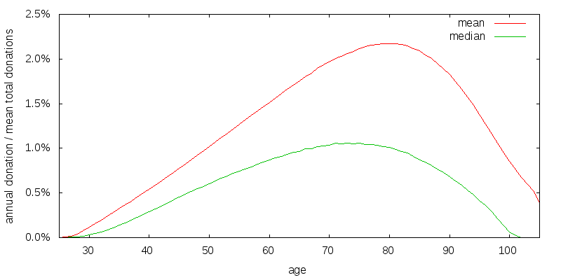
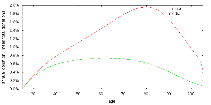
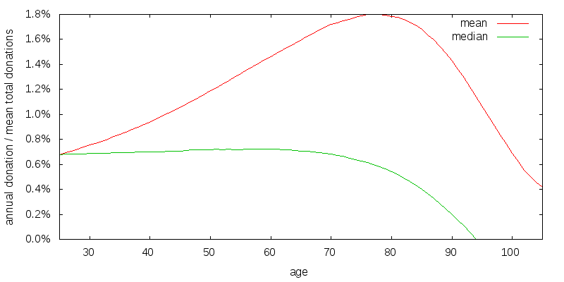
So far I have assumed a 6.5% arithmetic investment return with 22.2% volatility. Figure 15 presents the donation curves for a lower 2.9% investment return with 10.5% volatility such as might be expected from a 60/40 stock/bond asset allocation. The investment return is less than the donation rate, and the curves have shifted left.
So far I have assumed $100k per year of uncorrelated donations provided by third parties. Figure 16 shows the effect of reducing this amount to $10k. There is a greater need to provide for some consumption at all times, and the median consumption curve responds to this by flattening out.
So far I have been using a coefficient of relative risk aversion of consumption of 2. A reasonable value for the coefficient of relative risk aversion is probably somewhere in the range 1 to 4. Figure 17 shows the optimal strategy when donation and estate utility have a coefficient of relative risk aversion of 1.
Lower risk aversion has caused the width of the donation curve to shrunk somewhat compared to the baseline scenario.
Beyond simply the coefficient of relative risk aversion truly being 1, there are several additional reason to favor a reduced spreading out of donations:
So far utility has been based on purely altruistic motives. This is not always the case. I now switch to incorporating personal satisfaction from donating into the analysis. I do this by adding satisfaction utility to donation utility and estate utility to produce total utility.
Two things set satisfaction utility apart from donation and estate utility. First, satisfaction utility is not affected by experience. You are assumed to feel the same about donating a particular amount irrespective of how much you donated previously. Second, satisfaction utility does not normally undergo any discounting nor any increase due to knowledge. This is because you feel roughly the same about donating a particular amount irrespective of age or how much you know. This point is particularly significant.
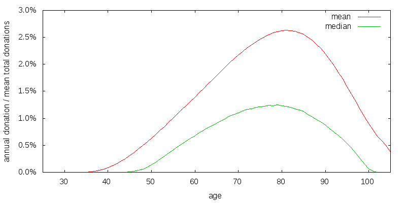
Figure 18 shows the effects of satisfaction on my baseline model. At early ages some donations are now occurring. This is a result of the model I use for satisfaction utility. Like estate and donation utility satisfaction is modeled using a CRRA utility function with a coefficient of relative risk aversion of 2, but instead of assuming $100,000 of uncorrelated "consumption", only $10,000 of consumption is assumed. This makes it more important that donations be non-zero at early ages.
The question "Who donates a constant amount?" has relevance since it seems like the default assumption that people might make. Indeed in the U.S. foundations are required to disburse a minimum of 5% per year, and for many this also becomes a maximum.
When discount rates are low you should donate late. When discount rates are high you should donate early. Returning to the satisfaction strategy of the previous section, there is a significant amount of donations are occurring from ages 80 to 100, although the chance of being alive through this period are increasingly small. This is because for reasons we have previously explained satisfaction isn't discounted. This means that at advanced ages even though satisfaction utility is small the amount of satisfaction that can be bought due to the compounding investment growth is large. Hence satisfaction skews things towards advanced ages. This can be corrected for as shown in Figure 19 by assuming satisfaction is discounted at a 4.0% rate. In addition I have removed the effects of experience and knowledge.
The lack of an experience and knowledge causes the strategy to start at a constant amount, satisfaction causes it to maintain a more or less constant amount, and the force of mortality eventually causes it to decline.
My model is built on one remotely possible and two unrealistic assumptions. The remotely possible assumption is the donation and estate discount rates are very close to the investment rate of return. The unrealistic assumptions are satisfaction is discounted at a relatively high rate. And little knowledge is gained over the first few decades. This answers the question: "Who, as a utility maximizer, should spend at a constant amount?".
Discounted satisfaction greatly changes the optimal spending strategy. Even though the spending curve changes markedly, overall utility changes far less. With the baseline scenario without experience or knowledge, 33.5e-6 units of utility are realized without satisfaction. Incorporating satisfaction with a 4.0% satisfaction discount rate 30.4e-6 units of donation and estate utility are produced and an additional 107.7e-6 units of satisfaction utility. By way of contrast the first strategy would have produced 77.6e-6 units of satisfaction had satisfaction been considered. In other extra satisfaction can be had for a small altruistic cost by spending at a near constant rate, provided that there is no experience or knowledge gain during the early years and satisfaction is discounted.
A spending strategy tells you how much to donate as a function of wealth and previous donation amount. It is thus possible to execute a spending strategy while applying an arbitrary set of utility functions and see how well it does using those utility functions. I do this using the near constant donation amount strategy of the last section. This allows us to answer the question: "What happens if utility is expressed according to the baseline utility functions, but we instead choose to follow the spend a near constant amount strategy?".
The baseline utility functions when executing the optimal strategy deliver 139.5e-6 units of utility. By contrast the baseline utility function when executing the previous spend at a near constant amount strategy delivers only 108.3e-6 units of utility. The optimal strategy provides an increase of 29%. This was for an estate and donation discount rate of 3% meaning that the optimal strategy is to spend late. Repeating the experiment with a 10% discount rate gave 32.2e-6 units of utility for the optimal strategy and 27.1e-6 units for spending a near constant amount, for an increase of 19%.
I was also interested in how the chosen investment strategy compares to a sub-optimal investment strategy. For a sub-optimal investment strategy I chose a 2.9% investment return with 10.5% volatility, indicative of a 60/40 stock/bond asset allocation. The optimal spending strategy for the sub-optimal investment strategy delivered 69.4e-6 units of utility. This represents a 101% increase for the chosen investment strategy. Repeating with a 10% discount rate gave 25.0e-6 units of utility for an increase in utility by 29%.
© 2016-2017 Gordon Irlam. Some rights reserved.
 This work is licensed under a Creative Commons Attribution-ShareAlike 4.0 International License.