Leveraged ETFs are entirely inappropriate for retirement investing, but may be useful for Effective Altruism investing. The volatility of leveraged ETFs is huge. Over the period 2007-2009, a 3X leveraged ETF would have likely fallen to 4% of its peak value. Losses of close to this magnitude are not extraordinary.
At present I would recommend investing in small cap value rather than leveraged ETFs. If investing in leveraged ETFs I would currently recommend the ProShares 2X leveraged ETF SSO. The ProShares 3X leveraged ETF UPRO has slightly better expected performance for effective altruism purposes, but this comes with higher volatility and an increased likely of negative results. This might lead to investor regret, and the possibility of bailing on the chosen strategy.
If investing in leveraged ETFs it is important to pay attention to expected returns on the underlying index, real borrowing costs, and the lag between leveraged ETFs and model leverage. The performance lag is made up of the expense ratio, overheads, and inefficiencies. When the key values change, so will the applicability of leveraged ETFs.
This article expands on Effective Altruism Investing Strategies by looking at the suitability of leveraged ETFs for effective altruism investments.
Effective altruism is a movement that seeks to use reason to achieve the most good in the world. The bulk of this article is relevant to anyone seeking a better understanding of the performance of leveraged ETFs. Only the final section deals with concerns specific to effective altruism.
Leverage is an advanced investing topic, and leverage should only be considered if you have mastered other aspects of investing, especially the potential permanently negative consequences of taking on risk.
Leveraged ETFs multiply the daily returns of an index; typically by a factor of 2 or 3. Leveraged ETFs return higher returns when times are good at the cost of worse returns when times are bad. Because the bet is recommitted to each day, over longer periods, the returns can be significantly higher than the factor of 2 or 3 that might be naively expected. This is also true for negative returns, and makes leveraged ETFs unsuitable for most investors.
The primary investment strategy of leveraged ETFs is the execution of swap agreements. These swap agreements are contracts that specify the ETF will pay a counterparty a fixed interest rate in exchange for receiving or making payments equal to the change in value of the index through some date. The counterparty is typically a large bank or brokerage that is able to at least notionally use the interest payments to borrow funds and then invest the funds in the stock market. The leveraged ETF will also hold cash pledged as collateral against the swap agreement, and may hold shares making up the underlying index (either directly or through shares in an ETF that tracks the underlying index), as well as possibly index futures contracts. The composition of these later components is likely to vary on a day-to-day basis to maintain the target leverage factor, while new swap agreements are probably only executed monthly, or less frequently.
The expected results for a leveraged ETF then are very similar to what you might expect if you borrowed on margin to invest in the market, and were rebalancing on a daily basis to maintain the target leverage factor. If you were to borrow funds you would likely pay a higher margin rate than a leveraged ETF, but on the flip side you don't have to deal with associated management expenses and other fund expenses, which for 3X funds are typically a high 0.95% per annum. This suggests a natural benchmark for a leveraged ETF: the daily return on the underlying total return index multiplied by the leverage factor less the cost of borrowing funds at the risk free rate. For the risk free rate I will normally be adopting the Fedfunds rate, which is the rate on overnight loans between banks. For long run historical analysis the Fedfunds rate isn't available, so I use the 1-month Treasury bill rate plus 0.4%, which is the difference between these two interest rates over the period 1955-2016.
For current analysis I use arithmetic mean annualized real stock market returns of 4.5% with an annualized real volatility of 16.8%. This corresponds to a geometric mean real return of 3.2%. These numbers are justified in Effective Altruism Investing Strategies. As of April 2017 the Fedfunds rate was 0.9% nominal, and the Survey of Professional Forecasters inflation projection for 2017 was 2.3%, resulting in a real cost of borrowing of -1.4%.
For historical analysis I use the return statistics of Dimson, Marsh and Staunton's Credit Suisse yearbook weighted developed world index for the period 1900-2016, with an arithmetic mean real annualized returns of 6.5%, and volatility 17.4%. The reported geometric mean is 5.1%. They also report the geometric mean real interest rate for short term Treasury bills as 0.8%, making the risk free rate 0.8% + 0.4% = 1.2%.
FINRA, the financial industry regulatory authority has put out an alert warning of the risks of leveraged ETFs to buy-and-hold investors. These products are entirely inappropriate for typical retirement portfolios, but the risk profile may be appropriate for effective altruists. In Effective Altruism Asset Allocation it was shown that a reasonable asset allocation for effective altruism portfolios is probably around 300% stocks.
Table 1 presents the available forward leveraged ETFs that are based on broad U.S. market indexes. Of the 2X ETFs, Direxion's SPUU has low assets, low volume, and tracks the index poorly, making ProShares' SSO preferable. Of the 3X leveraged ETFs ProShares' UPRO appears to lag an idealized benchmark by less than Direxion's SPXL. This makes UPRO preferable, with the caveat that Yahoo Finance was only able to provide two full years of financial data for UPRO with a computed lag of 1.3%, so I instead used seven full years of UPRO net asset values to compute the performance lag. SPXL provided eight years of data.
| ETF | leverage factor | performance lag | underlying index |
|---|---|---|---|
| ProShares SSO | 2 | 1.4% | S&P 500 |
| Direxion SPUU | 2 | 3.5% | S&P 500 |
| ProShares UPRO | 3 | 1.8% | S&P 500 |
| Direxion SPXL | 3 | 2.2% | S&P 500 |
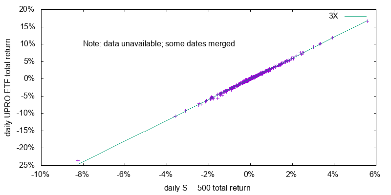
On a daily basis the return of leveraged ETFs do a good job of tracking the underlying index as shown in Figure 1. On an annual basis things are less attractive as the management fees, effective costs of borrowing, and other expenses add up.
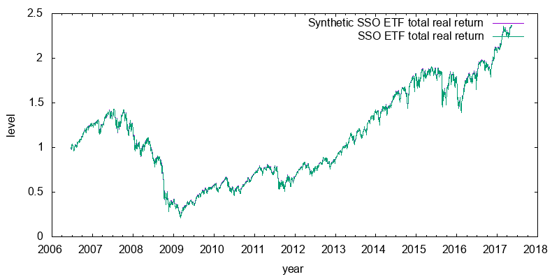
I model the level of a leveraged ETF using the applicable total return index, the leverage factor, the then Fedfunds rate, and a single fudge factor: the empirically derived annual lag of the ETF behind this benchmark. Figure 2 shows the performance of SSO against this model. I intentionally chose SSO, because it is the only leveraged ETF with financial data prior to the 2007-2009 sub-prime financial crisis. This is a period where the Fedfunds rate was much higher than it is today. The model tracks the actual data very closely. So closely that the two lines are largely coincident and you really have to peer at the graph before you can see any of the red line. Model versus actual plots for UPRO and SPXL are similar. SPUU does a worse job of tracking its model, although it still tracks it reasonably well.
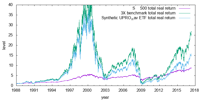
Daily data for the S&P 500 total return index is available from 1988 on. This suggests a natural backtest for UPRO, in which we calculate how the leveraged ETF would have been expected to perform. This is shown in Figure 3. Some observations are in order. First in a rising or declining market the gains are losses are far in excess of 3X. This is due to the daily resetting. Second the synthetic UPRO significantly lags its benchmark after 30 years due to the annual underperformance lag adding up. Third the synthetic UPRO hasn't regained the level it had during the 2000 dotcom bubble, despite the index having done so. Forth, whether the synthetic UPRO outperforms the simple 1X index depends on the ending date chosen, but overall on average it outperforms. Finally, from 2000 to 2002 the synthetic UPRO dropped to 7.3% of its peak value value, and from 2007 to 2009 it dropped to 4.2% of that peak value. For a synthetic 2X SSO the corresponding declines were to 19.9% and 15.5% of their peak values respectively. It takes a very strong mind to be able tolerate such losses.
The previous synthetic backtest is for a single history, and will not re-occur in the future. To predict performance in the future I construct a simple mathematical model of what is happening.
I assume the total return index can be described using geometric Brownian motion with constant drift, constant volatility, and no-autocorrelation. Later we will see how inaccuracies in this assumption lead to discrepancies between the mathematical model and bootstrapped projected performance.
In the presence of leverage, the geometric Brownian motion drift parameters μleverage_GBM and underlying volatility σleveraged_GBM would be expected to given by:
where μindex_GBM is the drift on the underlying total return index, σindex_GBM is the underlying total return index volatility, f is the leverage factor (2 or 3), RfGBM is the instantaneous risk free rate, and LagGBM is the instantaneous performance lag. These later two values are related to the annualized risk free rate, Rf, and the expense ratio and other factors related lag, Lag, by:
Geometric Brownian motion results in a log-normally distributed returns. Returns after n years are given by the lognormal probability density function with parameters μ = n . μLND, and σ = sqrt(n) . σLND. Or equivalently, the annualized return is given by the lognormal probability density function with parameters μ = μLND, and σ = σLND / sqrt(n). By comparing the definitions of geometric Brownian motion and the lognormal distribution it can be seen:
The parameters μLND and σLND of the log-normal distribution are given by the equations:
where R and σ are the arithmetic mean annual return and volatility respectively.
I thus proceed as follows. Compute μindex_LND and σindex_LND using equations (5) and (6). Convert them to μindex_GBM and σindex_GBM using equations (3) and (4). Compute the leveraged values μleveraged_GBM and σleveraged_GBM using equations (1) and (2). Convert these values back to μleveraged_LND and σleveraged_LND using equations (3) and (4) in reverse. Compute and plot the corresponding probability density function.
It is worth noting that the model is independent of the inflation rate. This can be seen by assuming the values used in the leverage equation are all nominal, and the instantaneous inflation rate is w, so that:
which is the leverage equation in real form, independent of the inflation rate.
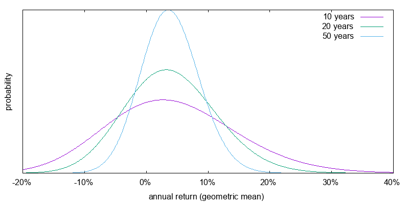
First we will apply the model to the present. Figure 4 shows projected return probabilities for a 3X ETF for different holding periods assuming a constant cost of borrowing of -1.4%. Even for a 50 year period there is a significant chance of -5% annual returns, which would result in the original investment being cut down to 8% of its original value. Worse annualized returns are possible over shorter periods.


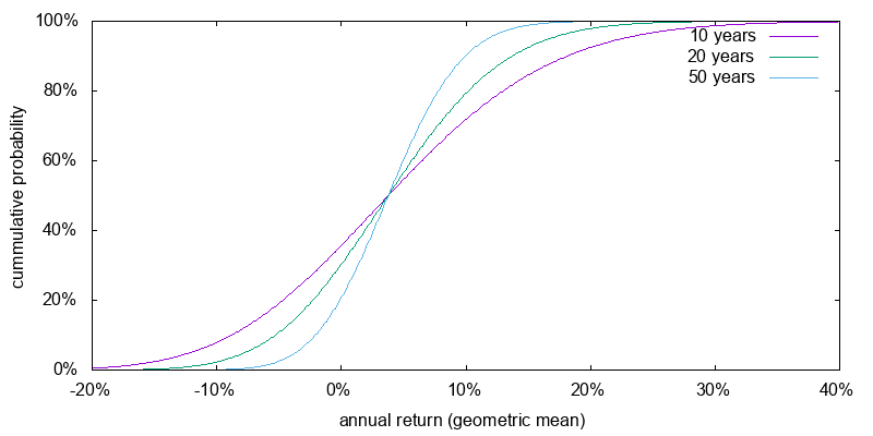
Now we turn to how the model performed using historical return statistics and borrowing costs. Figure 5 shows the return probabilities again for a 3X ETF. The return probabilities are very similar. Underlying index return expectations are higher, but this has largely been offset by higher borrowing costs.
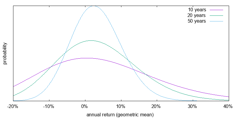
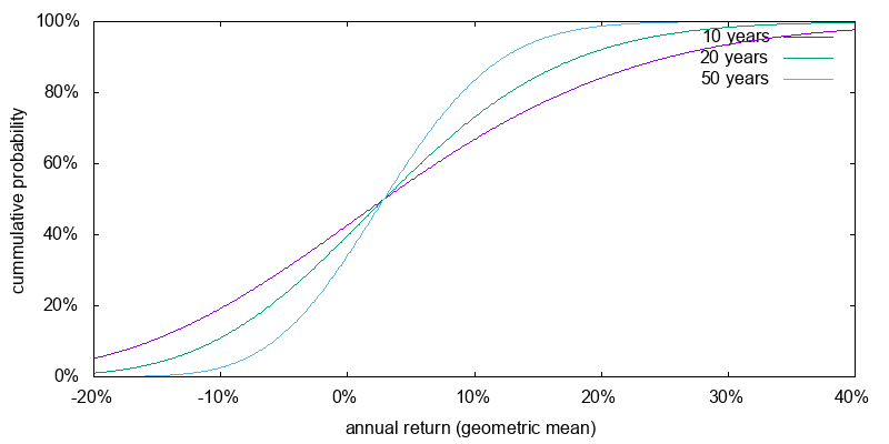
Figure 6 shows the return probabilities for a 2X ETF assuming the current projected market performance, cost of borrowing, and a 1.4% per annum performance lag, similar to that for SSO. The results can still be quite averse; less than in the 3X case, but perhaps still so bad that it doesn't make a lot of psychological difference. Decimation, even over 50 years, is still a possible outcome.
Bootstrapping is the technique of generating large amounts of return sequence data by concatenating smaller sub-sequences from the historical record. Unlike a mathematical model, bootstrapping allows the resulting return sequence to have variable drift, volatility, and auto-correlation phenomena such as momentum. Here I use bootstrapping to projected the performance of leveraged ETFs based on the daily S&P 500 total return index from 1988 to 2016, using only the leverage factor, the performance lag, and the risk free rate.
Since inflation is not uniform over this period, I subtract it out, and then add in an assumed constant inflation rate. Although, this later step isn't strictly necessary.
Since this is a relatively small time the mean annual return and volatility on an annual basis might differ substantially from the expected values. The next step then is to gently and uniformly massage the historical daily data so that it reflects the assumed annual return and volatility. To maximize the information contained in the data I compute annual returns using a 365 day wide sliding window (or strictly speaking 252 returns per year) and take the average value. I also wrap the data, joining the start of 1988 to the end of 2016 so that all data has equal weight, which helps with latter analysis.
Next I convert the daily return values into leveraged daily return values by using the leverage factor, the risk free rate, and the expected performance lag.
Finally I perform simulations. I construct 500000 return sequences. Each sequence is constructed by concatenating month long samples (21 returns per month) from within the wrapping leveraged daily return sequence. For each sequence I compute the final return value and plot a histogram of the results.
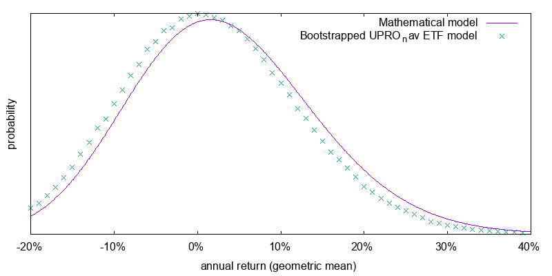
Figure 7 compares 20 year annualized returns of the mathematical model and the bootstrapped results, but with the underlying S&P 500 total return index replaced by an artificially generated true geometric Brownian motion sequence matching the assumed mean annual return and annualized volatility.
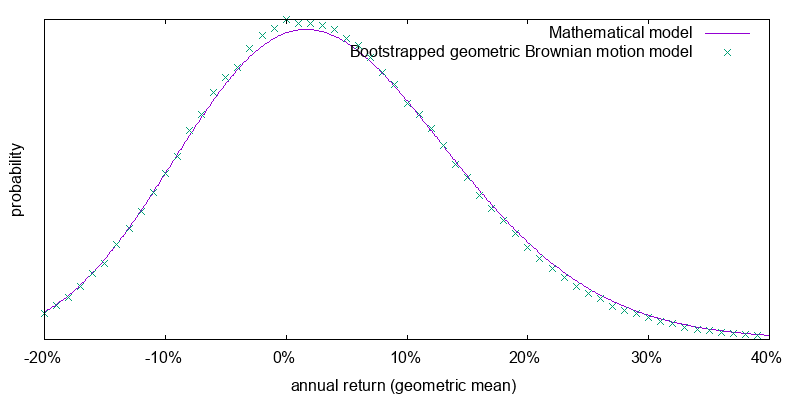
The good fit between the mathematical model and the bootstrapped results suggests we are on the right track. That the two do not fit perfectly can be ascribed to using month long samples in the bootstrapping process. I discovered that if I set the bootstrap sample size to one day the fit becomes perfect. I want to use a bootstrap sample size that is as large as possible so that when applied to real world returns it captures parameter variabilities and auto-correlations, but setting it too large means that the available samples do not reflect the full range of possibilities of true geometric Brownian motion. I found that when setting this sample size to two months or larger it started to reflect negatively on the tight relationship between the mathematical and geometric Brownian motion bootstrapped models. Hence the use of a one month sample size.
Figure 8 shows the application of the bootstrap model to the S&P 500 total return index. Here there is some divergence between the simple mathematical model that assumes geometric Brownian motion and the bootstrap model which does not, but the difference isn't that great. Using the bootstrap model is preferable, but we can probably get away with using the simple mathematical model if we need to.
Leveraged ETFs are highly volatile. This volatility could mistakenly lead to the conclusion that they are a poor ex-ante investment opportunity for effective altruism investing. It is therefore vital that before investing in them you know what to expect.
For the simple mathematical model the annual real volatility of a leveraged ETF can be calculated as:
This produces the volatilities shown in Table 2.
| asset allocation | σleveraged |
|---|---|
| 100% stocks | 22.2% |
| 200% stocks | 35.8% |
| 300% stocks | 58.6% |
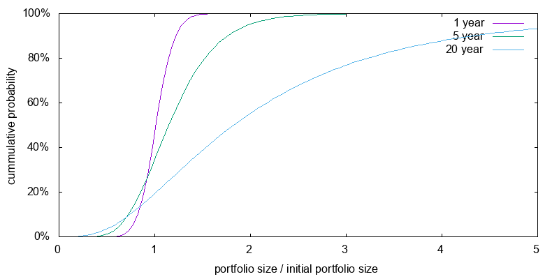
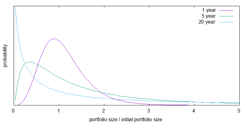
I turn now from the expected losses over a one year period to losses over multiple years, and switch from the simple mathematical model to the more accurate bootstrapped model. First, a basic understanding of the role of time on the value of investments is necessary. Figure 9 shows the projected distribution of relative portfolio sizes for an investment in an ETF that tracks the massaged S&P 500 index with a 0.1% expense ratio computed using the bootstrap model. As can be seen the greater the length of time, the greater the chance of major gains, while the chance of a major loss doesn't vary by much. A one year 20% loss isn't extraordinary.
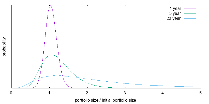
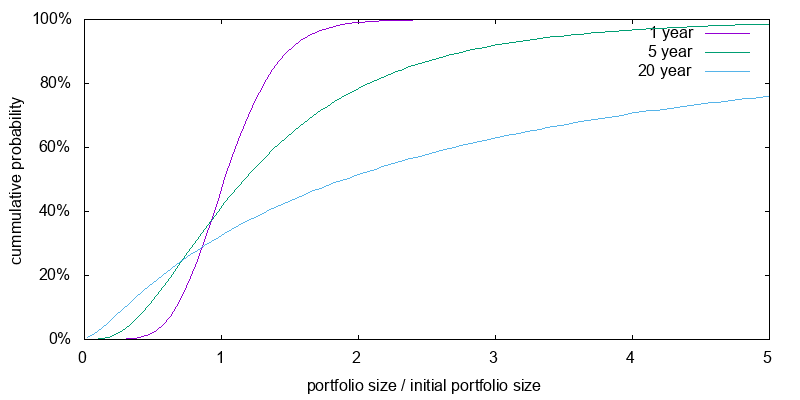
The same is not true when leverage is used. When leverage is used the chance of a major loss increases as time increases. A 40% one year loss isn't extraordinary. Figure 10 presents the current projected distribution of relative portfolio sizes for a 2X leveraged ETF investments after 1, 5, and 20 years using the bootstrap model and including an appropriate performance lag. As can be seen, the greater the duration, the higher the probability of a major loss, but also the higher the probability of major gains.
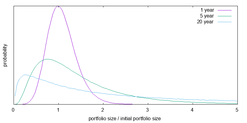
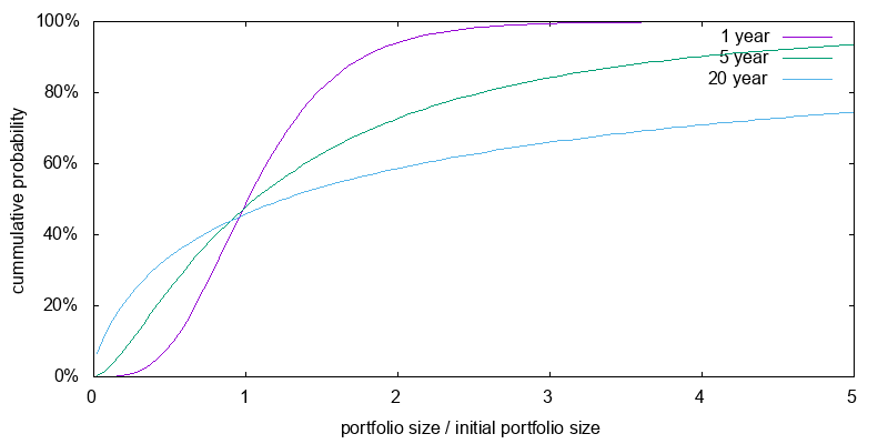
The corresponding graph for a 3X leveraged investment is shown in Figure 11. Here the chance of a major loss is very high especially as time increases. And even a one year 60% loss isn't extraordinary.
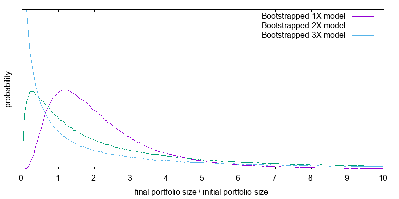
To reiterate the point, Figure 12 reproduces the 20 year results from the previous figures with a change in scale. Tables 3 and 4 present the median and mean final value factors for the above distributions. Leverage boosts the mean expected final portfolio size at the possible expense of median portfolio size. When you use leverage you are more likely to end up on the left of the graph, but you are hoping this will be offset by the small probability of ending at the extreme right. Be careful of fixating on expected mean final portfolio sizes. Utility, not wealth is what matters, and it displays diminishing marginal returns.
| asset allocation | 1 year | 5 year | 20 year |
|---|---|---|---|
| 100% stocks | 1.04 | 1.17 | 1.85 |
| 200% stocks | 1.05 | 1.19 | 1.92 |
| 300% stocks | 1.04 | 1.11 | 1.38 |
| asset allocation | 1 year | 5 year | 20 year |
|---|---|---|---|
| 100% stocks | 1.04 | 1.23 | 2.30 |
| 200% stocks | 1.08 | 1.48 | 4.74 |
| 300% stocks | 1.13 | 1.83 | 11.09 |
If the amount of good done was linear in donation amount, we would be done, but it is not. Because of the law of diminishing returns, the good done by a donation ten times as large is less than ten times the good done by a donation of a particular size. This is captured by the concept of utility.
In Effective Altruism Asset Allocation I suggest a reasonable model of utility for an individual is a constant relative risk aversion (CRRA) utility function with a coefficient of relative risk aversion of 2. However things become more complicated for an effective altruist because only a fraction of consumption is likely to be correlated with the returns of the optimal level of market leverage, while the rest can be treated as uncorrelated. I suggest that for every $100k per year of uncorrelated consumption, there might be somewhere around $200k of assets dedicated to the cause whose returns are correlated with the optimal level of market leverage. As it turns out the exact coefficient of relative risk aversion, and the exact amount of correlated assets doesn't matter greatly. What matters most is the is some uncorrelated consumption that acts as a brake on the worst aspects of a CRRA utility function at small levels of consumption.
My model of effective altruism utility then is to use the empirical bootstrapped model of leveraged ETF performance, each month to donate a fraction of the portfolio to the cause, and compute the utility associated with having done so. When computing utility I also take into account uncorrelated donations/consumption. At the end of each simulation sequence I add up all the utilities, and compute the total utility associated with that simulation sequence. Having done this it is possible to plot the range of utilities, or compute their median or mean. Since utility values are not meaningful to people, each utility is inversed to compute a certainty equivalence: the constant annual would be correlated donation amount that has the same utility as the given utility value.
In deciding how much to donate each year I keep things simple and used 1/N of the portfolio size where N is the number of years remaining. This is clearly sub-optimal. The optimal fraction is a function of both portfolio size and years remaining that varies in ways that can only be computed using stochastic dynamic programming. My attempt to use a slightly more sophisticated scheme, variable percentage withdrawal, which attempts to divide donations more uniformly by taking into account the growing nature of the portfolio, produced worse results; possibly because the extreme volatility of leveraged ETFs makes the growth rate to use hard to determine.
I developed an asset allocator called Opal that uses stochastic dynamic programming to determine the optimal asset allocation as a function of age and portfolio size. Opal can also be run in non-stochastic dynamic programming mode to compute the certainty equivalent utility associated with a given initial portfolio size and fixed asset allocation. Table 5 presents a comparison of the results produced using Opal and the bootstrap model. Simulation is a random process, and the variability associated with donation amounts reported by each model is in the range $100-200. Thus the two models are in good agreement.
| asset allocation | donation strategy | lag | annual certainty equivalent donation amount | |
|---|---|---|---|---|
| Opal | bootstrap model | |||
| 100% stocks | 1/N | 0% | $12,008 | $12,109 |
| 200% stocks | 1/N | 0% | $27,983 | $28,235 |
| 300% stocks | 1/N | 0% | $33,067 | $33,326 |
| 400% stocks | 1/N | 0% | $27,919 | $28,046 |
| optimal dynamic | 1/N | 0% | $36,719 | - |
| optimal dynamic | optimal dynamic | 0% | $40,409 | - |
| optimal dynamic | optimal dynamic | 1.8% | $31,374 | - |
There are three additional lines in the above table that were computed using stochastic dynamic programming, and against which no bootstrap model comparison is available. They show a reasonable gain in performance if the asset allocation is allowed to vary dynamically. A further gain in performance if the donation strategy is chosen to be optimal, as a function of portfolio size and time, rather than 1/N. And a significant drop when a typical leveraged ETF performance lag exists.
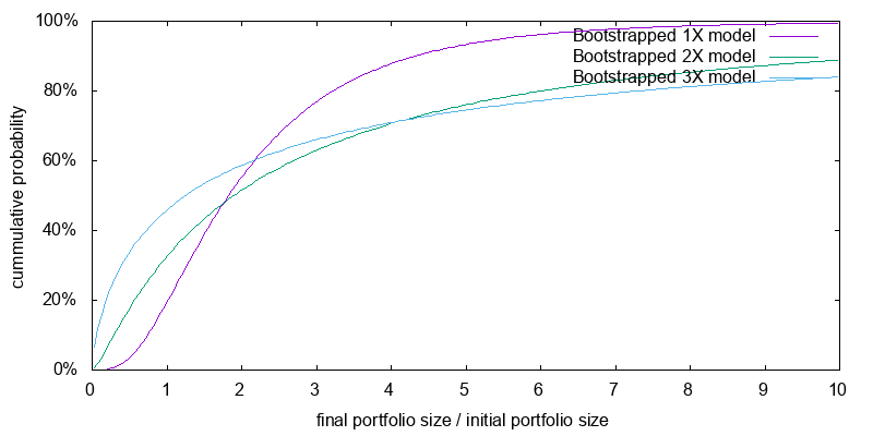
Figure 13 presents the distribution of certainty equivalent values for the current time scenario, 1/N donating, and a 20 year time horizon. This plot incorporates the performance lag between the leverage benchmark and an actual leveraged ETF. The associated summary statistics are presented in Table 6. It is easy to see the case for 2X leverage of effective altruism resources. It boosts both the median and the mean donation amount. The case for 3X is harder to see as the mean is boosted, but the median falls. It is quite likely that you will end up with a smaller value than with 2X, but there is a small chance it will be significantly larger boosting the mean. Despite this the case has been made since our preferences over different donation levels are captured by the concept of utility, and effective altruists may not be mean donation amount maximizers, but should be mean utility maximizers. Beyond 3X, no case can be made. Both the mean and median fall.
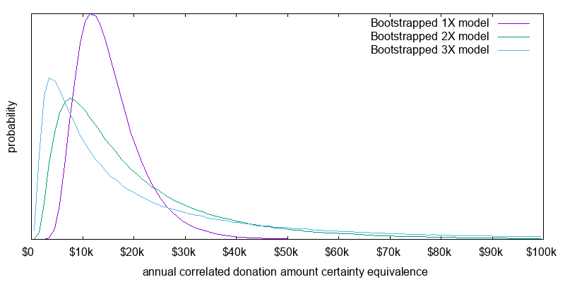
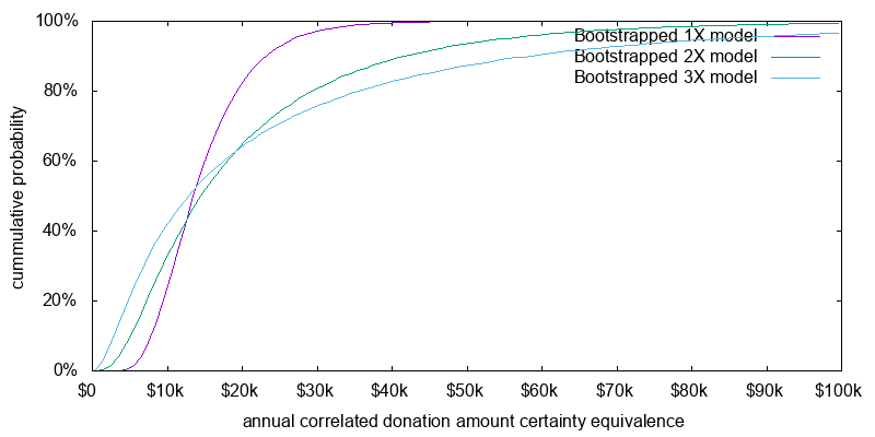
| asset allocation | annual certainty equivalent donation amount | |
|---|---|---|
| median | mean | |
| 100% stocks | $14,002 | $14,901 |
| 200% stocks | $15,035 | $18,452 |
| 300% stocks | $13,334 | $19,528 |
| 400% stocks | $9,388 | $17,224 |
| 100% small cap value (no anomaly) | $15,849 | $17,384 |
| 100% small cap value (anomaly) | $24,103 | $25,658 |
The gains from leverage are far smaller than those seen in the validation section, which saw a doubling or tripling of the certainty equivalent mean donation amount. There are two reasons for this. First the results in the validation section were for 50 years rather than 20 years, giving more time for advantages to compound. Second the lag between idealized leverage performance and actual leverage performance exerts a significant toll. 1.8% per year over 20 years is a 30% drag.
Also note the comparison against small cap value computed both on a purely risk adjusted basis (no anomaly), and as if there is a future 4% small and value performance anomaly (anomaly). Depending on whether you believe there is an anomaly small cap value comes reasonably close to performing as well as leverage, or significantly exceeds the performance of leverage. This is quite different from the results computed in Effective Altruism Asset Allocation where fixed and dynamically variable leverage both outperformed anomaly free small cap value by a wide margin. The likely reason for this difference is the other paper assumes idealized leverage without the performance lag of leveraged ETFs seen in the real world.
Based on the previous two sections mathematically speaking a 3X leveraged ETF, such as UPRO, currently has a small advantage over 1X or 2X for effective altruism purposes, but it may be wise to use a 2X leveraged ETF, such as SSO, owing to the significantly reduced downside of doing so. Investing in the 2X ETF would probably make it slightly easier to sleep at night. That said, both options are only just superior, or significantly inferior to investing in small cap value, depending on whether there are persistent small and value performance anomalies.
Important reasons the results contained here might not be valid include:
Leveraged ETFs lag idealized benchmarks by 1.4% to 2.2% per year. A better understanding of the components of this lag is in order. Expense ratios and other fund expenses typically add up to around 0.95% per year. There is also the interest rate margin on the fund borrowing for the swap contract, which needs to be multiplied by the leverage factor. But with sufficient assets I would have thought this could have been negotiated to a low value. Perhaps there are other cost factors of which I am unaware.
It would be informative to know if leveraged ETF swap contracts are pegged to the basic index, or the total return index. My analysis was based on the total return index less some lag. An alternative analysis based on the basic index plus some margin is also possible. The iPath SFLA exchange traded note is indexed against the S&P 500 total return index, suggesting swap contracts indexed to the total return index are possible.
Data was sourced from Fred, Yahoo Finance, and ProFunds. It was analyzed using a 700 line Python program called Leverage Analyze. For performance reasons it should normally be run using the PyPy just-in-time Python compiler. Data was plotted using the leveraged_etfs.gnuplot GnuPlot script. The simple mathematical model was generated using the investing_math_model.py Python program and plotted using the investing_math_model.gnuplot GnuPlot script.
© 2017 Gordon Irlam. Some rights reserved.
 This work is licensed under a Creative Commons Attribution-ShareAlike 4.0 International License.